Hebbian Links
Now I am going to mention one of the great names in neurology, the person whose research probably kicked off the whole field of trying to recreate neural activity in computers, Donald Hebb. He was a neurologist working in the forties and fifties who developed the concept of Hebbian Learning and Cell Assemblies. His seminal work was Organization of Behaviour, in which he outlined these theories. At the time of publication (1949), they were only theories, but they have since been supported by a great deal of neurological evidence.
This has been phrased into a rather pithy saying, which I wish I'd thought of (but didn't):
"Cells that fire together, wire together!"
The simple theory of Hebbian Learning was later expanded to include Anti-Hebbian learning, in which any connection from cell A to cell B will weaken if only one of the cells fires. This effect is often called Long-Term Depression (LTD) and it opens the way up to two possibilities:
In fact, Hebb went beyond the idea of connections altering. He proposed that individual neurons or groups of neurons would spontaneously hook themselves up to form reverberating networks: neuron A would activate neuron B, which activates neuron C which then reactivates neuron A again. A circuit like this would get round the problem of the fact that neurons fatigue (they grow tired the longer they are active). This was Hebb's idea of Cell Assemblies, and which are a complete area of research in themselves! Using Hebb's idea of connections strengthening with use and weakening with non-use, we can model a simple Hebbian connection (also called a Hebbian link) between two neurons. What we are modelling is not the neurons themselves, but the strength of the connection between them, so an individual connection boils down to one floating point number - what could be simpler? Of course, you can't get much of a performance from just one connection, so we might as well model a whole bunch of them in one go. The sort of situation where you would have such a Hebbian net might be like the following: Imagine that your input was a grid of 5 squares by 5 squares. On to this grid were placed one of two images, representing a (crudely drawn) happy face, and a sad face: 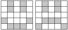 We want a Hebbian net to distinguish between these two faces, so we need one output, which will be 1 for the happy face, and 0 for the sad face. There should be a Hebbian link between all 25 input elements and the single output. In a later example, we will see how to adapt this when there is more than one output. This single output is shown in the diagram below: 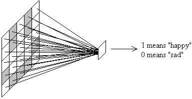 The entire Hebbian net is modeled simply by 25 numbers, each of which starts off with some random weight value, say between 0 and 1:
The function Math.rand() returns a random number in the range 0 to 1 (including the possibility of 0 but not of 1). In a language such as C++, you would need to change this to something similar to random(1000)/1000.0. Note the .0 on that to avoid the problem of integer division, which would always gives the answer 0. Having set up the connections, they must be trained. Put an input pattern on the input, the desired output pattern that it is supposed to produce on the output and then adjust the strengths of the connections appropriately. This leads to a slight problem - the exact nature of the training rule. If we just take Hebb's idea of connections strengthening, without worrying about them weakening again, then we use the generalised Hebb rule: Δw = η.ai.aj
In this case, Δw is the change in the weight connecting input element i to output element j. ai is the activation of input element i and aj is the activation of output element j. η is constant term that prevents the changes in the weight from being too extreme. For example, suppose that a weight from an input neuron to an output neuron is currently 0.75. Suddenly an input and output pattern are presented, and the input element has activation of 0.5 and the output element has an activation of 0.2. If the constant η is 0.01, then the weight is changed (increased) by the value of 0.5 x 0.2 x 0.01 = 0.001. This means that the weight increases from 0.75 to 0.751. Here is the code for updating all the weights for the happy/sad face example. I assume that the input pixels are stored in an array ipt[] and the single output element (0 or 1) is given by opt:
Of course, providing that the inputs and outputs are always 0 or greater, the weights can never decrease, they can only ever increase. This is where the generalised Hebbian rule can be extended. If the formula above is changed to the following: Δw = η.(2ai - 1).aj
then the weight will be decreased whenever the activation of input i is less than 0.5. This is because (2ai - 1) will produce a negative number. However, the value of aj will still always be positive. This situation is called Post-not-pre LTD as it means that the strength will be reduced whenever the input neuron (the "pre-synaptic neuron") is asleep but the output neuron (the "post-synaptic neuron") is awake. The formula could also be written the other way round: Δw = η.ai.(2aj - 1)
In this case, the weight is reduced whenever the input neuron is active but the output neuron is inactive, i.e. it is Pre-not-post LTD. You might be tempted to go one stage further and incorporate both types of LTD in one formula: Δw = η.(2ai - 1).(2aj - 1)
but a moment's thought reveals this to be silly. In this case, if both the input and the output neurons were off (i.e. had activation 0 or some low activation - certainly lower than 0.5), then the two negative numbers produced would multiply to give a positive number, and the weight would actually increase! Just stick to one or the other, whichever one gives you the best results. Here is the adapted code which updates the strengths. I have included a variable which specifies the "training type", i.e. whether the strengths are to be updated using LTP only (the generalised Hebb rule), Post-not-pre LTD or Pre-not-post LTD:
One question is, "Should the weights be limited to the range 0 to 1?" There is nothing in Hebb's rule that says weights can't increase indefinitely, and nothing in the LTD rules to say that they can't become negative. If you did want to constrain them, you could add lines of code that make sure they never go outside the range 0 to 1:
Don't forget to call the update_strengths procedure many times, so that the strengths can adjust to their final values. In the following code, I have not defined the procedure copy_input, but this simply copies training pattern number pattern to the array inp[].
Generally, Hebbian networks learn very slowly. You will find you have to present input patterns many times (often thousands of times) to make them learn correctly, and even then they don't always get it right! If you have, say, 8 training patterns (possibly 4 happy faces and 4 sad ones), then you would present each face with its appropriate output to the net in turn, update the weights, then repeat that for the other 7 faces, and then repeat the whole procedure as many times as are needed. Running the networkHaving set up the connections, you now want to run the network to see if it can correctly classify the happy and sad face pictures that it has been trained upon. This involves putting the test pattern at the inputs, multiplying each of the input elements by the weight of its connection and adding up the results. This will produce an answer for the output, which will probably not be exactly 0 or 1, but will hopefully be close to one or the other. If the answer is above 0.5, then the net has classified the face as happy (i.e. output = 1). If less than 0.5, then that means sad (i.e. output = 0):
Two-dimensional Hebbian networksIt is a fairly easy matter to extend the output to two dimensions as well as the input. In this case, the simple output variable, opt, is replaced by an array opt[] which represents an output grid: 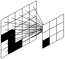 In this diagram, I have only shown the connections to one output element as including them all would make the diagram too cluttered. Since all the output elements are connected to all the input elements, the strengths[] array now has to have 4 dimensions, not 2. In this case strengths[a][b][c][d] would represent the strength of the connection between element [a][b] of the input pattern to element [c][d] of the output pattern. Apart from that, the code would be very similar to that of the previous example:
You see that the output grid needn't be the same size (or even the same shape) as the input pattern. In this case, I am assuming that the output grid is 3-by-3 and the input is 5-by-5. The only real major change is the routine that runs the net. In this case, we can't simply sum the weighted inputs to produce a final answer, as the answer will come out as a grid of numbers. We have to take the grid of numbers that is produced and comapre it with all the desired outputs from the training patterns to see which one is the closest. That desired output pattern then represents the neural network's choice. What do the egg-heads say about Hebbian links?You want to read Hebb's original book? It's rather dull, I must warn you. He has also written other things since 1949. I happen to know he was already a fully-fledged professor in 1949 - imagine how old he must have been in 1980! |
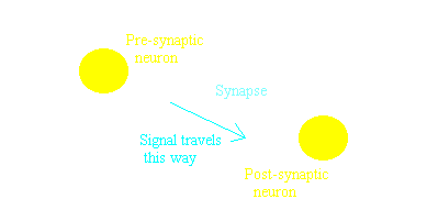 The idea of Hebbian learning concerns how the synaptic connection from one neuron to another strengthens, allowing a larger signal to pass from one neuron to the next. In short, Hebb proposed that if there is a synaptic connection from cell A to cell B, and both cells happen to fire at the same time (perhaps as a result of cell A passing a signal to cell B), then the synaptic connection between the cells becomes stronger. This will mean that cell A will be more likely to cause cell B to fire in future. An analogy might be a muscle becoming stronger, the more it is used. This strengthening of the connection is sometimes referred to as Long-term Potentiation (LTP) in the literature