The Kohonen Self-Organising Map

This architecture was pioneered by Professor Teuvo Kohonen at the University of Helsinki. It is unlike the other architectures that we have met before as it involves unsupervised training. It learns the patterns for itself without being told what it is supposed to be learning!

In supervised learning, which is what we have been using up to now, we train the networks by presenting them with an input pattern together with a corresponding output pattern, and the networks adjust their connections so as to learn the relationship. However, with the Self-Organising Map (SOM), we just give it a series of input patterns, and it learns for itself how to group these together so that similar patterns produce similar outputs.

It's about time that we saw for ourselves what the SOM looks like ....

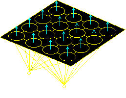
Well, that's the Kohonen SOM on the right. It consists of a single layer of cells, all of which are connected to a series of inputs. The inputs themselves are not cells and do no processing - they are just the points where the input signal enters the system.

The cells in the diagram appear to have connections between them (and indeed, descriptions of Kohonen nets I have read generally refer to "lateral inhibitory connections"), but the algorithm for training the net never mentions them, and so, I shan't refer to them again!

Training the Kohonen SOM

The SOM is generally speaking a two-dimensional structure - a rectangular grid of cells - which allows "blobs" of activity to appear on its surface and represent groupings. If it were three dimensions or more, then it would be hard for anyone to visualise the patterns of activity.

However, for the purposes of describing the training algorithm, I shall use a one-dimensional example. The idea behind the training is that the weights (strengths of connections between the inputs and each of the nodes in the grid) are set to random values. Then the patterns are presented one after each other. Each pattern is "run forward" in the net, so that the net produces an output.

Although the weights are random, one of the nodes has to produce a slightly higher output than the others, and that node is chosen as the "winner." The weights of the winning node and those in its immediate neighbourhood are updated slightly so that they are more likely to correspond to the input pattern in future. In this way, groups of nodes across the SOM become dedicated to classes of input pattern and those similar to them.

Initialise the network
Let's say that w_ij is the weight from input number i to cell number j. We will also assume that there are n input values, and number them from 1 to n.

These weights are set up to be small random values. No reference paper has ever told me exactly how small "small" is, so I tend to make them very small, i.e. some random number in the range 0 to 0.01. We also have to decide upon the size of the neighbourhood of each cell, which we call for cell j, N. This is set to a large value (typically almost the size of the entire grid). I have chosen to implement the size in terms of a radius, i.e. a distance from the central winning node.
```
var n = 2;         // How many inputs
var NUMCELLS = 10; // How many cells in grid

var radius;        // Distance of influence from any cell
var w = new Array();   // Weights from "n" inputs to NUMCELLS outputs
for (var i = 0; i < n; i++)
  w[i] = new Array();
// w[i][j] = weight from input "i" to node "j"

function initialise ()
{ for (var i = 0; i < n; i++)
   for (var j = 0; j < NUMCELLS; j++)
    w[i][j] = Math.random() * 0.01;   // Range 0 to 0.01
}
```
Present input
Present the first input pattern, which we call x₁ to x_n, where x_i is the input to node i. We don't seem to need to run the network forward, as far as I can see.

var x = new Array(); // Contains input
Calculate distances
Calculate the distances between the input and each of the output nodes in turn. We produce a distance figure for each cell j, and do it by going through all the inputs and adding the squares of the differences between the input value and the weight (yes, I kid you not - the weight, not the output value!). As an equation, this is written as follows:

d_j = n-1
S
0 (x_i - w_ij)²

and if you prefer that in non-gobbledy gook,
```
var d = new Array();   // contains differences

for (var j = 0; j < NUMCELLS; j++)
 { d[j] = 0;
   for (var i = 0; i < n; i++)
    d[i] += (x[i] - w[i][j]) * (x[i] - w[i][j]);
       // This last part squares x[i] - w[i][j]
 }
```

Select the minimum distance

Find the cell with the minimum difference, and call that node j^*

var j_star, temp_d;

temp_d = 10000;     // Set temp_d to a dummy high distance value
for (var j = 0; j < NUMCELLS; j++)
 if (d[j] < temp_d)    // Bound to happen sooner or later
  { temp_d = d[j];
    j_star = j;
  }

Update the weights
Update the weights for node j^* and all the nodes in the same neighbourhood (as defined by the size of N). New weights are given by the following formula

new w_ij = old w_ij + h(x_i - w_ij)

The weights that are not in the neighbourhood are not changed at all. h is a gain term between 0 and 1 which decreases slowly over time, thereby slowing down the rate at which weights adapt. The size of the neighbourhood, N also decreases slowly as time goes on, thus localising the area of maximum activity. Unfortunately, Kohonen and those that have come after him have stated that there are "no hard and fast rules" determining how quickly and at what point these values should decrease.
Repeat the process
Repeat the process by going back to step 2. You should present different input patterns cyclically (no, not using ESP, just cycle through the patterns: 1, 2, 3, 1, 2, 3 etc.) and at regular intervals (undefined) reduce the neighbourhood size and gain term. The convergence does seem to be rather slow - typically a few hundred cycles should happen before these sizes are reduced at all.

Running the Kohonen SOM

This part I have never seen in any literature about SOMs - not once. Nobody seems to write about it, so I have had to work out the rule for myself. However, it does seem to work.

To calculate the output for each cell, just apply the required input to all the nodes. Then, for each cell in the grid, multiply corresponding inputs and weights, and sum the values, and that is the output for that node. There doesn't seem to be any need for a transfer function.

for (var j = 0; j < NUMCELLS; j++)
 { var sum = 0.0;
   for (var i = 0; i < n; i++)
    sum += w[i][j] * x[i];  // Weight times input
   alert('Output for cell ' + j + ' : ' + sum);
 }

We can't guarantee that the output of the cells will be in the range 0.0 to 1.0. It may be above 1.0, so there may be occasions where you have to impose a ceiling on it. In the example below, I artificially impose a ceiling of 1.0 so that the pictures are displayed correctly.

An example of a Kohonen SOM

This example shows a JavaScript version of the one-dimensional SOM that I have just described. It has 10 output cells and two inputs. During training, the program is designed to present two types of input to the SOM, either the first input high (in the range 0.8 to 1.0) and the second low (0.0 to 0.2) or vice-versa.

Two inputs:

Initial range (2-4)

Iterations

The way you use the program is as follows: Firstly (without training the net), try a few values in the range 0 to 1 in the two input slots on the left. You should find that the network doesn't give much of a response, since the weights are initially very low. Then click on the Train button, and repeat the testing process. You should find that you get well defined islands of activity when the first input is high (0.8 to 1.0) and the second low (0 to 0.2) or vice-versa.

A two-dimensional Kohonen SOM

The Kohonen SOM really comes into its own with a two-dimensional grid of cells. The example I have included below is similar to the one dimensional example except that all the variables have been given the suffix '2' to distinguish them from the variables in the one-dimensional example. For instance, the weights are stored in the array w2. However, the input still uses the array x.

This time the input consists of four groups of numbers: Low-low, Low-high, High-low and High-high, created in the same manner as before. We should find that four large "islands" of activation form in the grid, although we can't predict exactly where.

Two inputs:

Initial range (2-4)

Iterations

N.B. Some academic literature refers to the SOM as a Self-Organising Feature Map (SOFM), so consider this alternative name when you search for them with a search engine.